In the last post, I explored how to get below disributions with incanter.

• Uniform distribution
• Exponential distribution
• Beta distribution

Incanter supports various distributions: (From: http://incanter.github.io/incanter/distributions-api.html)

• beta-distribution
• binomial-distribution
• chisq-distribution
• exponential-distribution
• f-distribution
• gamma-distribution
• integer-distribution
• neg-binomial-distribution
• normal-distribution
• poisson-distribution
• t-distribution
• uniform-distribution

But Scipy stats supports lot more distributions.
In JVM world, there’s another library that supports various distributions called Apache Commons Math, and here are list of distributions supported by the library. In order to make those distributions available from Incanter world, I’ve created small library called incanter-contrib-distribution.

Below are some of the examples of how to use it.

• Cauchy distribution
• Gamma distribution
• Triangular Distribution

Cauchy distribution

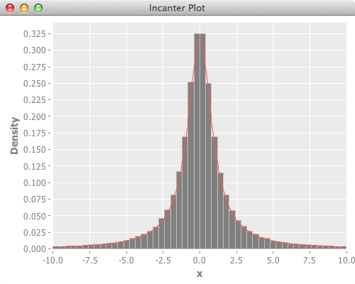
PDF of Cauchy distribution:


(From http://en.wikipedia.org/wiki/Cauchy_distribution)

Cauthy distribution has wide support, so for plotting, filtered out values out of certain range.

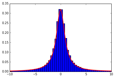
Below is the reference scipy version, and it’s plot.

1
2
3
4
5
6
7
8
9
10
11
12
13
14
15
16
17

import numpy as np
from scipy.stats import cauchy
import matplotlib.pyplot as plt

np.random.seed()
N = 100000
rv = cauchy(loc=0.0, scale=1.0)
x = rv.rvs(size=N)
x = x[(x>-10) & (x<10)]
nbins = 50
plt.hist(x, nbins, normed=True)

x = np.linspace(-10, 10, 1000)
plt.plot(x, rv.pdf(x), 'r-', lw=2, label='cauchy pdf')
plt.xlim((-10, 10))

plt.show()

Gamma distribution

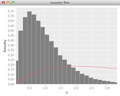
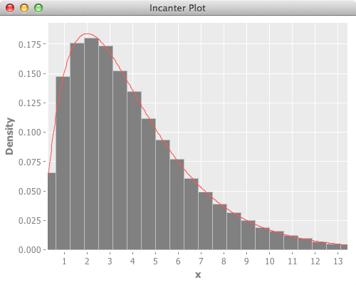
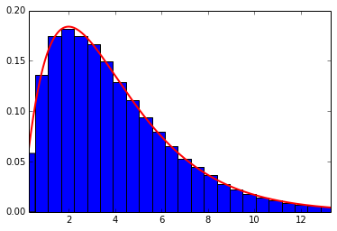
PDF of Gamma Distribution:


(From http://en.wikipedia.org/wiki/Gamma_distribution)

Gamma distribution exists in incanter, but in incanter-1.5.5, there’s still issue around draw.
Here’s how it’s not properly working with incanter-1.5.5 gamma-distribution.

Though this was fixed in issue#245 and is available in head, I used incanter-contrib-distributions for this for now.

Below is the reference scipy version, and it’s plot.

1
2
3
4
5
6
7
8
9
10
11
12
13
14
15
16

import numpy as np
from scipy.stats import gamma
import matplotlib.pyplot as plt

np.random.seed()
N = 100000
rv = gamma(a=2.0, scale=2.0)
x = rv.rvs(size=N)
nbins = 50
plt.hist(x, nbins, normed=True)

x = np.linspace(rv.ppf(0.01), rv.ppf(0.99), 1000)
plt.plot(x, rv.pdf(x), 'r-', lw=2, label='uniform pdf')
plt.xlim((rv.ppf(0.01), rv.ppf(0.99)))

plt.show()

Triangular Distribution

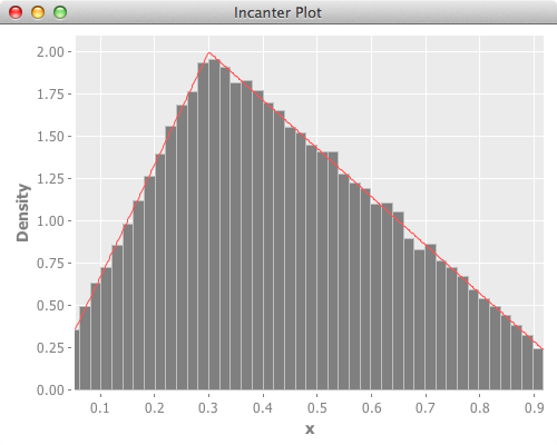
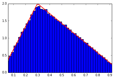
PDF of Triangular Distribution:


(From http://en.wikipedia.org/wiki/Triangular_distribution

Below is the reference scipy version, and it’s plot.

1
2
3
4
5
6
7
8
9
10
11
12
13
14
15
16

import numpy as np
from scipy.stats import triang
import matplotlib.pyplot as plt

np.random.seed()
N = 100000
rv = triang(loc=0.0, c=0.3, scale=1.0)
x = rv.rvs(size=N)
nbins = 50
plt.hist(x, nbins, normed=True)

x = np.linspace(rv.ppf(0.01), rv.ppf(0.99), 1000)
plt.plot(x, rv.pdf(x), 'r-', lw=2, label='triang pdf')
plt.xlim((rv.ppf(0.01), rv.ppf(0.99)))

plt.show()