I was looking for ways to get random numbers from various distributions in Clojure.Incanter .
Below are the list of distributions mentioned in this page.
Through out this page, I used below project.clj.
(defproject various-distributions "0.1.0-SNAPSHOT"
  :description "FIXME: write description"
  :url "http://example.com/FIXME"
  :license {:name "Eclipse Public License"
            :url "http://www.eclipse.org/legal/epl-v10.html"}
  :dependencies [[org.clojure/clojure "1.6.0"]
                 [incanter/incanter-core "1.5.5"]
                 [incanter/incanter-charts "1.5.5"]]
  ;; :jvm-opts ^:replace []
  :main ^:skip-aot various-distributions.core
  :target-path "target/%s"
  :profiles {:uberjar {:aot :all}})
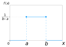
Probability density function(PDF) of Uniform Distribution:http://en.wikipedia.org/wiki/Uniform_distribution_(continuous) )
(ns various-distributions.uniform
  (:require [incanter.charts :as c]
            [incanter.core :as i]
            [incanter.distributions :as d]))

(defn show-uniform-distribution []
  (let [dist (d/uniform-distribution 0.0 1.0)
        n 10000
        x (repeatedly n #(d/draw dist))
        pdf-fn #(d/pdf dist %)]
    (let [nbins 50
          series-label "uniform"]
      (-> (c/histogram x :nbins nbins :density true :series-label series-label)
          (c/add-function pdf-fn 0 1 :series-label "uniform-pdf")
          i/view))))
This is pretty straight forward.
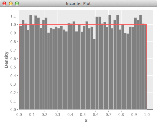
Here’s the plot. Red line is theoretical value.
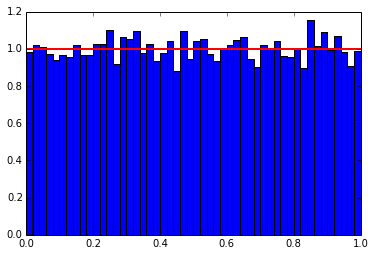
Below is the reference scipy version, and it’s plot.
1
2
3
4
5
6
7
8
9
10
11
12
13
14
15
import numpy as np
from scipy.stats import uniform
import matplotlib.pyplot as plt
np . random . seed ()
N = 10000
rv = uniform ( loc = 0.0 , scale = 1.0 )
x = rv . rvs ( size = N )
nbins = 50
plt . hist ( x , nbins , normed = True )
x = np . linspace ( rv . ppf ( 0 ), rv . ppf ( 1 ), 100 )
plt . plot ( x , uniform . pdf ( x ), 'r-' , lw = 2 , label = 'uniform pdf' )
plt . show ()
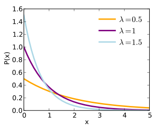
PDF of Exponential Distribution:http://en.wikipedia.org/wiki/Exponential_distribution )
(ns various-distributions.exponential
  (:require [incanter.charts :as c]
            [incanter.core :as i]
            [incanter.distributions :as d]
            [incanter.stats :as s]))

(defn show-exponential-distribution []
  (let [dist (d/exponential-distribution 1.0)
        n 100000
        x (repeatedly n #(d/draw dist))
        pdf-fn #(d/pdf dist %)]
    (let [nbins 50
          series-label "exponential"
          [x-min x-max] (s/quantile x :probs [0.01 0.99])]
      (-> (c/histogram x :nbins nbins :density true :series-label series-label)
          (c/set-x-range x-min x-max)
          (c/add-function pdf-fn x-min x-max :series-label "exponential-pdf")
          i/view))))
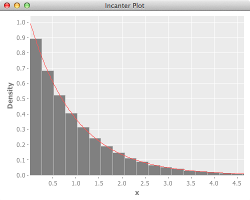
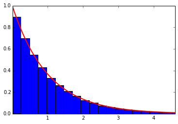
Since incanter didn’t have ppf(Percent point function, inverse of cdf), I used percentile of the created random values to get lower and upper range for drawing plot.
Below is the reference scipy version, and it’s plot.
1
2
3
4
5
6
7
8
9
10
11
12
13
14
15
16
import numpy as np
from scipy.stats import expon
import matplotlib.pyplot as plt
np . random . seed ()
N = 100000
rv = expon ( scale = 1.0 )
x = rv . rvs ( size = N )
nbins = 50
plt . hist ( x , nbins , normed = True )
x = np . linspace ( rv . ppf ( 0.01 ), rv . ppf ( 0.99 ), 1000 )
plt . plot ( x , rv . pdf ( x ), 'r-' , lw = 2 , label = 'uniform pdf' )
plt . xlim (( rv . ppf ( 0.01 ), rv . ppf ( 0.99 )))
plt . show ()
http://en.wikipedia.org/wiki/Beta_distribution )
(ns various-distributions.beta
  (:require [incanter.charts :as c]
            [incanter.core :as i]
            [incanter.distributions :as d]
            [incanter.stats :as s]))

(defn show-beta-distribution []
  (let [dist (d/beta-distribution 2 5)
        n 100000
        x (repeatedly n #(d/draw dist))
        pdf-fn #(d/pdf dist %)]
    (let [nbins 50
          series-label "gamma"
          [x-min x-max] (s/quantile x :probs [0.01 0.99])]
      (-> (c/histogram x :nbins nbins :density true :series-label series-label)
          (c/set-x-range x-min x-max)
          (c/add-function pdf-fn x-min x-max :series-label series-label)
          i/view))))
1
2
3
4
5
6
7
8
9
10
11
12
13
14
15
16
import numpy as np
from scipy.stats import beta
import matplotlib.pyplot as plt
np . random . seed ()
N = 100000
rv = beta ( a = 2.0 , b = 5.0 )
x = rv . rvs ( size = N )
nbins = 50
plt . hist ( x , nbins , normed = True )
x = np . linspace ( rv . ppf ( 0.01 ), rv . ppf ( 0.99 ), 1000 )
plt . plot ( x , rv . pdf ( x ), 'r-' , lw = 2 , label = 'uniform pdf' )
plt . xlim (( rv . ppf ( 0.01 ), rv . ppf ( 0.99 )))
plt . show ()
References
Helpful references were:

