More Distributions With Incanter and Commons Math
In the last post, I explored how to get below disributions with incanter.
Incanter supports various distributions: (From: http://incanter.github.io/incanter/distributions-api.html)
- beta-distribution
- binomial-distribution
- chisq-distribution
- exponential-distribution
- f-distribution
- gamma-distribution
- integer-distribution
- neg-binomial-distribution
- normal-distribution
- poisson-distribution
- t-distribution
- uniform-distribution
But Scipy stats supports lot more distributions.
In JVM world, there’s another library that supports various distributions called Apache Commons Math, and here are list of distributions supported by the library.
In order to make those distributions available from Incanter world, I’ve created small library called incanter-contrib-distribution.
Below are some of the examples of how to use it.
Cauchy distribution
PDF of Cauchy distribution:


(From http://en.wikipedia.org/wiki/Cauchy_distribution)
Cauthy distribution has wide support, so for plotting, filtered out values out of certain range.
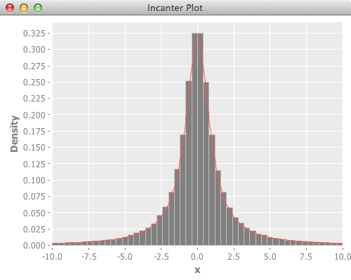
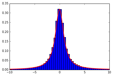
Below is the reference scipy version, and it’s plot.
1 2 3 4 5 6 7 8 9 10 11 12 13 14 15 16 17 | |
Gamma distribution
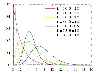
PDF of Gamma Distribution:

(From http://en.wikipedia.org/wiki/Gamma_distribution)
Gamma distribution exists in incanter, but in incanter-1.5.5, there’s still issue around draw.
Here’s how it’s not properly working with incanter-1.5.5 gamma-distribution.
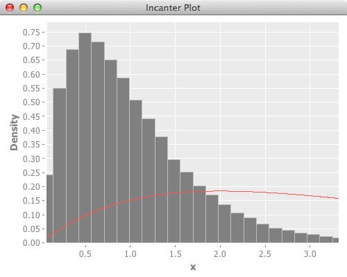
Though this was fixed in issue#245 and is available in head, I used incanter-contrib-distributions for this for now.
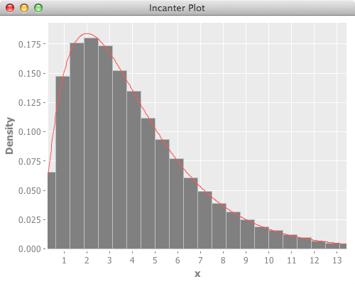
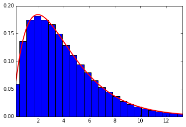
Below is the reference scipy version, and it’s plot.
1 2 3 4 5 6 7 8 9 10 11 12 13 14 15 16 | |
Triangular Distribution
PDF of Triangular Distribution:


(From http://en.wikipedia.org/wiki/Triangular_distribution
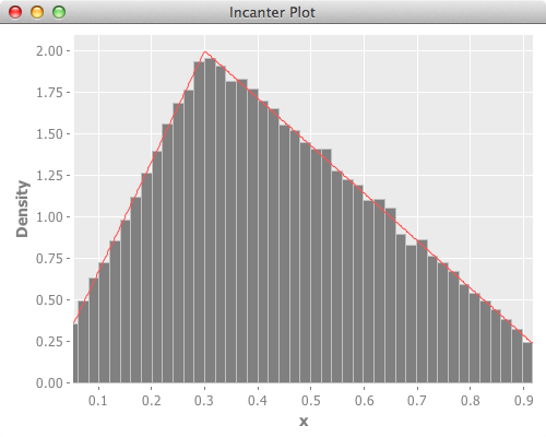
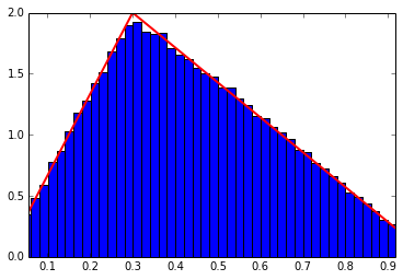
Below is the reference scipy version, and it’s plot.
1 2 3 4 5 6 7 8 9 10 11 12 13 14 15 16 | |
Various Distributions With Incanter
I was looking for ways to get random numbers from various distributions in Clojure.
Here’s how I got it with Incanter.
Below are the list of distributions mentioned in this page.
Through out this page, I used below project.clj.
Uniform distribution
Probability density function(PDF) of Uniform Distribution:

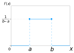
(From http://en.wikipedia.org/wiki/Uniform_distribution_(continuous))
This is pretty straight forward.
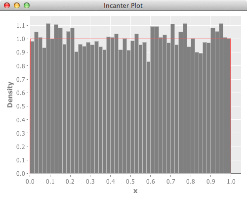
Here’s the plot. Red line is theoretical value.
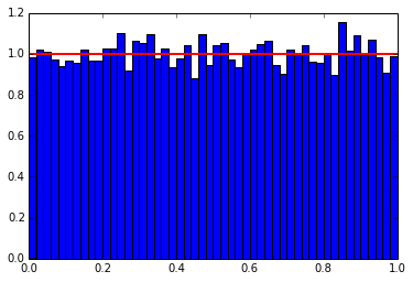
Below is the reference scipy version, and it’s plot.
1 2 3 4 5 6 7 8 9 10 11 12 13 14 15 | |
Exponential distribution
PDF of Exponential Distribution:

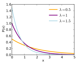
(From http://en.wikipedia.org/wiki/Exponential_distribution)
Since incanter didn’t have ppf(Percent point function, inverse of cdf), I used percentile of the created random values to get lower and upper range for drawing plot.
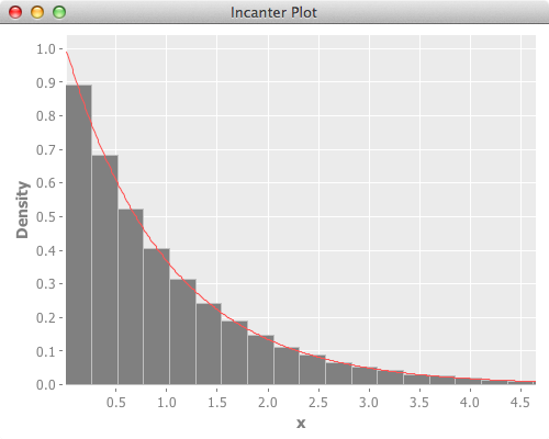
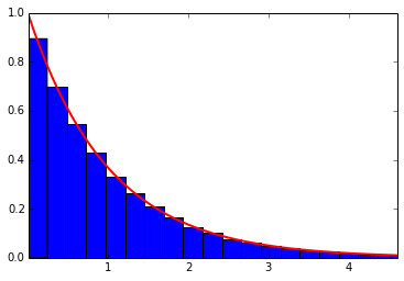
Below is the reference scipy version, and it’s plot.
1 2 3 4 5 6 7 8 9 10 11 12 13 14 15 16 | |
Beta distribution


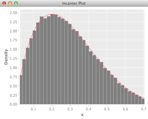
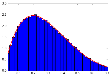
(From http://en.wikipedia.org/wiki/Beta_distribution)
1 2 3 4 5 6 7 8 9 10 11 12 13 14 15 16 | |
References
Helpful references were:
http://aidiary.hatenablog.com/entry/20140620/1403272044
This person was doing similar thing in python.